Visualize neural recordings#
VneuroTK’s viz extra provides Matplotlib plots of stimulus timing and neural activity. It is separate from vneurotk.vision, which extracts representations with deep neural network (DNN) vision models.
Prerequisites: install VneuroTK with the visualization and notebook extras, for example uv add "vneurotk[viz,notebook]". This guide is offline and uses deterministic synthetic data.
Plot continuous data with BaseData.plot#
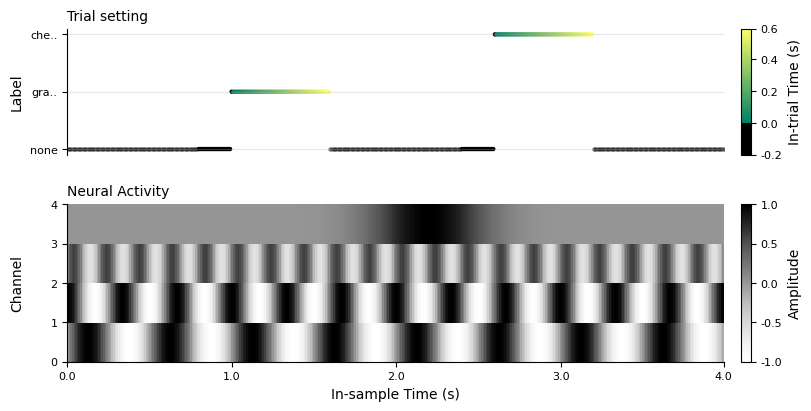
Create a sampled recording, configure stimulus onsets, and ask the data object to build the standard two-panel figure. The upper panel shows trial labels and relative trial time; the lower panel is a channel-by-time heatmap.
import numpy as np
from loguru import logger

import vneurotk as vtk

logger.remove()

t = np.arange(400) / 100.0
continuous_neuro = np.column_stack(
    [
        np.sin(2 * np.pi * 2 * t),
        np.cos(2 * np.pi * 3 * t),
        0.6 * np.sin(2 * np.pi * 5 * t + 0.4),
        np.exp(-(((t - 2.2) / 0.35) ** 2)),
    ]
)
continuous = vtk.BaseData.for_continuous(
    continuous_neuro,
    neuro_info={"ch_names": ["V1", "V2", "V3", "V4"], "sfreq": 100.0},
)
continuous.configure(
    stim_ids=["grating", "checkerboard"],
    vision_onsets=np.array([100, 260]),
    trial_window=[-20, 60],
)

continuous_figure = continuous.plot(window=(0, 400), figsize=(8, 4))
continuous_figure
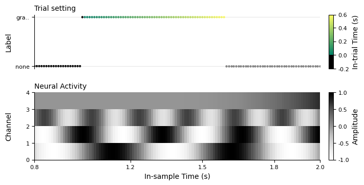
window=(0, 400) uses integer sample indices. Non-integral real bounds use seconds, so window=(0.8, 2.0) selects the same kind of interval in physical time. Keep the numeric types intentional: 2 means sample 2, while 2.0 means 2 seconds.
seconds_figure = continuous.plot(window=(0.8, 2.0), figsize=(7, 3.5))
seconds_figure
Plot pre-epoched data#
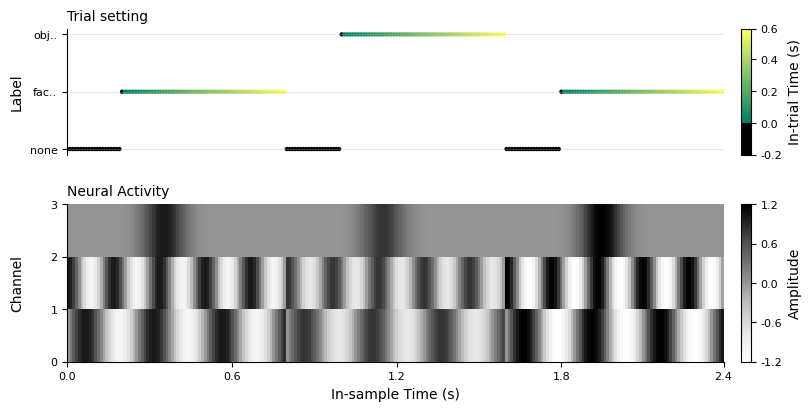
BaseData.plot also accepts epochs mode. It flattens the trial and time axes for display while preserving each trial’s configured onset and label.
epoch_time = np.arange(80) / 100.0
base_epoch = np.column_stack(
    [
        np.sin(2 * np.pi * 4 * epoch_time),
        np.cos(2 * np.pi * 6 * epoch_time),
        np.exp(-(((epoch_time - 0.35) / 0.08) ** 2)),
    ]
)
epoch_neuro = np.stack([base_epoch, 0.8 * base_epoch, 1.2 * base_epoch])
epochs = vtk.BaseData.for_epochs(
    epoch_neuro,
    neuro_info={"ch_names": ["occipital", "temporal", "parietal"], "sfreq": 100.0},
)
epochs.configure(
    stim_ids=["face", "object", "face"],
    vision_onsets=np.array([20, 20, 20]),
)

epoch_figure = epochs.plot(window=(0, 240), figsize=(8, 4))
epoch_figure
Call vneurotk.viz.plot_data directly#
Use the lower-level function when arrays are not wrapped in BaseData. neuro must be samples by channels, and visual must provide one stimulus label (or None) per sample.
labels = np.full(len(t), None, dtype=object)
labels[100:160] = "grating"
labels[260:320] = "checkerboard"

direct_figure = vtk.viz.plot_data(
    neuro=continuous_neuro,
    visual=labels,
    sfreq=100.0,
    window=(80, 200),
    figsize=(7, 3.5),
    cmap_neuro="Blues",
    color_offtime="0.35",
)
direct_figure
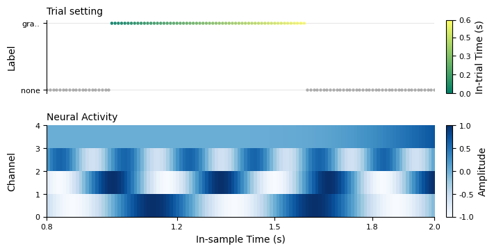
Figure ownership and supported data#
Both APIs create and return a Matplotlib Figure; the caller owns it. Keep the return value to annotate or save it, and call plt.close(figure) when a script no longer needs it. Notebook display keeps these figures open so their committed PNG output remains visible.
Visualization is limited to recordings with a time axis: continuous and epoched data. patterns mode contains aggregated rows rather than time samples, so BaseData.plot() rejects it.