Synthetic evoked-response visualization workflow#
This example builds a continuous recording with repeatable evoked responses, configures stimulus trials and baseline timing, and produces overview, focused, and customized Matplotlib figures.
Prerequisites: install vneurotk[viz,notebook]. Everything below is deterministic and offline. The viz module plots neural recordings; it does not run the DNN vision models provided by vneurotk.vision.
Synthesize a recording#
The signal combines low-amplitude oscillations with a stimulus-locked Gaussian response. Two stimulus categories use different channel profiles, making their evoked activity visible without downloading data.
import numpy as np
from loguru import logger

import vneurotk as vtk

logger.remove()

sfreq = 100.0
n_samples = 700
times = np.arange(n_samples) / sfreq
onsets = np.array([120, 330, 540])
stim_ids = np.array(["face", "object", "face"])
channel_profiles = {
    "face": np.array([1.0, 0.7, 0.2, -0.3, -0.6, -0.2]),
    "object": np.array([0.2, 0.5, 1.0, 0.7, 0.1, -0.4]),
}

neuro = np.column_stack(
    [0.08 * np.sin(2 * np.pi * (2.0 + 0.35 * channel) * times + 0.3 * channel) for channel in range(6)]
)
for onset, stimulus in zip(onsets, stim_ids, strict=True):
    latency = (np.arange(n_samples) - onset) / sfreq
    response = np.exp(-0.5 * ((latency - 0.22) / 0.07) ** 2)
    neuro += response[:, None] * channel_profiles[stimulus][None, :]

recording = vtk.BaseData.for_continuous(
    neuro,
    neuro_info={
        "ch_names": ["O1", "Oz", "O2", "PO3", "POz", "PO4"],
        "sfreq": sfreq,
    },
)
Configure stimuli and baseline#
The integer trial window [-20, 70] spans 20 baseline samples before each onset and 70 samples after it. At 100 Hz, the derived baseline is −0.20 to 0 seconds and the full trial is −0.20 to 0.70 seconds.
recording.configure(
    stim_ids=stim_ids,
    vision_onsets=onsets,
    trial_window=[-20, 70],
)
recording.trial_info
{'baseline': [-20, 0], 'trial_window': [-20, 70]}
Inspect the full experiment#
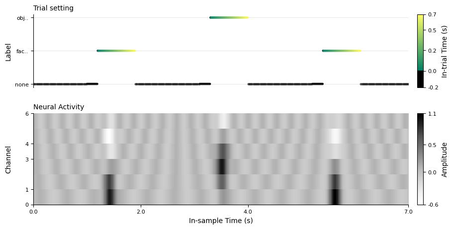
Integer display bounds are sample indices. The overview includes all three configured trials.
overview_figure = recording.plot(window=(0, 700), figsize=(9, 4.5))
overview_figure
Focus on one evoked response#
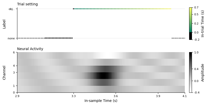
Non-integral float bounds are seconds. This 2.9–4.1 second view isolates the object trial while retaining its baseline and response.
focused_figure = recording.plot(window=(2.9, 4.1), figsize=(8, 4))
focused_figure
Customize and annotate the returned axes#
BaseData.plot returns an ordinary Matplotlib figure. Pass plotting options through the method, then find the neural-activity axis and add domain-specific annotations. The figure remains caller-owned for further edits, saving, or closing.
custom_figure = recording.plot(
    window=(4.9, 6.2),
    figsize=(8, 4),
    cmap_neuro="RdBu_r",
    cmap_ontime="viridis",
    color_offtime="0.45",
    marker_size=55,
)
neural_axis = next(axis for axis in custom_figure.axes if axis.get_title(loc="left") == "Neural Activity")
stimulus_time = onsets[-1] / sfreq
neural_axis.axvline(stimulus_time, color="#A23B72", linewidth=1.5, linestyle="--")
neural_axis.annotate(
    "stimulus onset",
    xy=(stimulus_time, 5.7),
    xytext=(stimulus_time + 0.12, 5.25),
    arrowprops={"arrowstyle": "->", "color": "#A23B72"},
    color="#6F2450",
    fontsize=9,
)
custom_figure
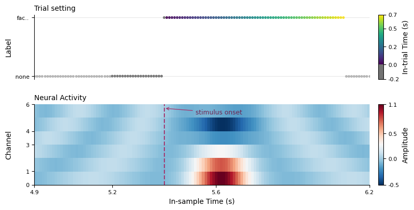
The overview establishes experiment structure, the focused view checks one trial in detail, and the custom view demonstrates Matplotlib-level extension without transferring figure ownership away from the caller.